Jennica Sandberg
Jennica Sandberg
Jennica Sandberg
Drug Discovery -Predicting Potential Antivirals
Drug Discovery -Predicting Potential Antivirals
Drug Discovery -Predicting Potential Antivirals
A Machine Learning Pipeline targeting SARS-CoV-2 Inhibition.
A Machine Learning Pipeline targeting SARS-CoV-2 Inhibition.



Python
Python
ChEMBL API
PaDEL-Descriptor
Bioinformatics
Regression Models
Published October 2024
Headquarters
Finland
Output
Streamlined Drug Discovery Workflow
Target-Specific Analysis
Data-Driven Insights
industry
Biotechnology
GitHub Repo
About the project
About the project
This bioinformatics project centers on developing a machine learning workflow to predict the bioactivity of compounds targeting specific proteins associated with SARS-CoV-2 — particularily focusing on viral inhibition for coronavirus strains. This project aims to create a scalable framework for bioactivity prediction using machine learning and bioinformatics tools, looking at small molecule inhibitors for effective treatment of SARS-CoV-2.
I selected ‘coronavirus’ as the target search keyword and chose the Replicase polyprotein 1ab, CHEMBL4523582. This enzyme is crucial for viral replication because it processes the polyproteins that the virus needs to replicate within host cells. Inhibiting this protease can potentially halt or slow down viral replication, making it a prime target for drug discovery efforts aimed at COVID-19 treatments. Studies have demonstrated that compounds targeting this protease can effectively disrupt the virus's ability to replicate, leading to ongoing research into its inhibition as a therapeutic strategy against coronavirus infections (Kandagalla et al., 2022 , Rhamadianti et al., 2024).
This case study follows a structured pipeline as follows:
Data Collection: Retrieving bioactivity data for CHEMBL4523582 using the ChEMBL API.
Data Preprocessing: Cleaning and transforming the data, calculating the Lipinski descriptors.
Exploratory Data Analysis (EDA): Utilizing chemical space analysis techniques to examine patterns in the dataset, particularly analyzing molecular properties.
Feature Engineering: Calculating molecular descriptors and fingerprints with PaDEL-Descriptor to enchance predictive modeling.
Model Development: Building and evaluating several regression models, with primary focus on Random Forest Regression, to predict compound bioactivity levels.
Results Analysis: Assessing model performance, comparing algorithms, and examining insights generated from these predictions.
This project ultimately serves as a comprehensive case study on bioactivity prediction that showcases a pipeline integrating data collection, bioinformatics and machine learning to explore potential apporoaches in drug discovery. As the pipeline is adaptable, it can be used for other targets or disease areas based on user input. The full instructions how to use the scripts are documented in the README.md file in the GitHub repo.
Visit Github
Development
Development
Technology Stack
Technology Stack
Python
Python
pandas
pandas
padelpy
padelpy

RDKit
RDKit

numpy
numpy

seaborn
seaborn
matplotlib
matplotlib

ChEMBL API
ChEMBL API
Git
Git
GitHub
GitHub

VS Code
VS Code
Data Collection
Data Collection
Using Python and the ChEMBL API I fetched compound bioactivity data related to a specific target protein associated with SARS-CoV-2, CHEMBL4523582. I chose this target as it is the latest single protein variant associated with SARS-CoV-2, making it interesting for studying potential antiviral compounds. The bioactivity data related to compounds interacting with the target protein was then filtered for IC50 to narrow down the focus to inhibitory effects.
The main.py script automates the retrieval process by querying ChEMBL’s database to collect the necessary bioactivity data and preprocesses it to clean and structure it for model input. Furthermore, based on the IC50 values the compounds are classified according to their bioactivity class, “inactive”, “intermediate”, and “active”.
By automating these data preprocessing steps, this process is reproducible, obtaining reliable input for the regression models, and ensuring that we get consistent data quality.
Data Preprocessing
Data Preprocessing
The next step in refine the collected data to improve the quality, which involved cleaning, transforming and engineering features using the analytics.py script. One of the key transformations was calculating Lipinski descriptors for each compound in the dataset. These assess the drug-like capacity of the compound measuring molecular weight (MW), lipophilicity (LogP), hydrogen bond donors and acceptors (NumHDonor, NumHAcceptor) as outlined by Lipinski’s Rule of Five.
IC50 values are also converted to logarithmic form (pIC50) to help normalize data distribution, and outliers were capped at 100,000,000 nM. Here the “intermediate” bioactivity class was also removed to ensure a clearer distiction between bioactive and inactive compounds.
Exploratory Data Analysis
Exploratory Data Analysis
In the Exploratory Data Analysis phase, I wrote the eda.py script to examine the structure and distribution of the data to identify patterns and relationships between inactive and active compounds. A frequency plot to show the distribution and a scatter plot to explore the relationship between MW and LogP.
Each Lipinski descriptor was then compared between active and inactive compounds using box plots, which visually help indentify any differences in distribution. To statistically validate these observations, I conducted Mann-Whitney U tests for each descriptor. This non-parametrics test allowed me to confirm whether there were statistically significant differences in descriptor values between active and inactive compounds. Here’s a summary of the findings:
| Descriptor | p-value | Distribution |
|---|---|---|
| pIC50 | 8.15 x 10^-130 | Different distribution |
| NumHDonors | 0.0033 | Different distribution |
| LogP | 2.15 x 10^-8 | Different distribution |
| NumHAcceptors | 0.4647 | No significant difference |
| MW | 0.4917 | No significant difference |
These results indicate that chemical properties, like pIC50, hydrogen donors, and LogP, likely influence compound activity, while molecular weight and hydrogen acceptors may play less of a distinguishing role in this dataset.
These results indicate that chemical properties, like pIC50, hydrogen donors, and LogP, likely influence compound activity, while molecular weight and hydrogen acceptors may play less of a distinguishing role in this dataset.
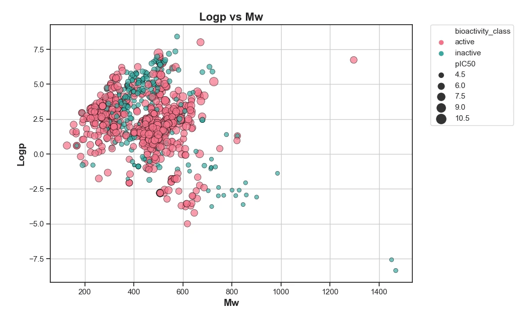


Figure 1: Scatter plot of LogP vs Molecular Weight (MW) for analyzed compounds. This plot illustrates the distribution of compounds based on their lipophilicity (LogP) and molecular size (MW). Compounds with a balanced LogP and optimal MW are often more favorable in drug discovery as they are more likely to have good absorption and distribution properties. Here, the spread of points indicates the variability in compound characteristics within the dataset.
Figure 1: Scatter plot of LogP vs Molecular Weight (MW) for analyzed compounds. This plot illustrates the distribution of compounds based on their lipophilicity (LogP) and molecular size (MW). Compounds with a balanced LogP and optimal MW are often more favorable in drug discovery as they are more likely to have good absorption and distribution properties. Here, the spread of points indicates the variability in compound characteristics within the dataset.
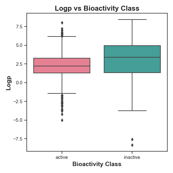


Figure 2: Distribution of LogP values in active vs. inactive compounds. This plot reveals a statistically significant difference between the compounds, as indicated by the rejection of the null hypothesis (H0). The spread and median LogP values suggest that LogP may influence bioactivity, with active compounds displaying distinct LogP characteristics compared to inactive ones.
Figure 2: Distribution of LogP values in active vs. inactive compounds. This plot reveals a statistically significant difference between the compounds, as indicated by the rejection of the null hypothesis (H0). The spread and median LogP values suggest that LogP may influence bioactivity, with active compounds displaying distinct LogP characteristics compared to inactive ones.
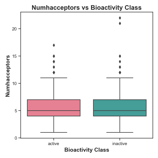


Figure 3: Distribution of NumHAcceptors in active vs. inactive compounds. The statistical test yielded no significant distribution, which can also be seen here, as both classes seem to be quite similar.
Figure 3: Distribution of NumHAcceptors in active vs. inactive compounds. The statistical test yielded no significant distribution, which can also be seen here, as both classes seem to be quite similar.
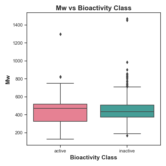


Figure 4: Distribution of Molecular Weight (MW) in active vs. inactive compounds. Since the null hypothesis (H0) was not rejected, there is no statistically significant difference in MW between the two bioactivity classes.
Figure 4: Distribution of Molecular Weight (MW) in active vs. inactive compounds. Since the null hypothesis (H0) was not rejected, there is no statistically significant difference in MW between the two bioactivity classes.
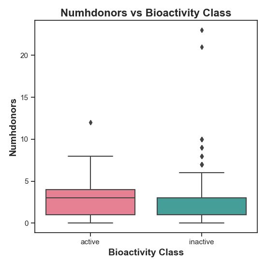


Figure 5: Distribution of NumHDonors in active vs. inactive compounds. There is a statistically significant difference in NumHDonors between the two bioactivity classes, meaning they have different distribution.
Figure 5: Distribution of NumHDonors in active vs. inactive compounds. There is a statistically significant difference in NumHDonors between the two bioactivity classes, meaning they have different distribution.
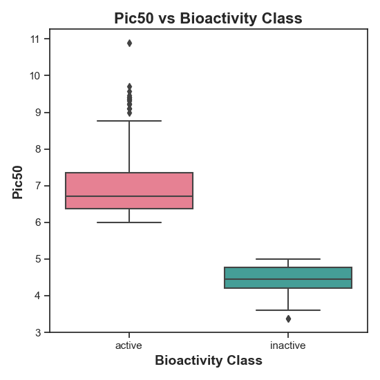


Figure 6: pIC50 Distribution across Bioactivity Classes. The rejection of the null hypothesis (H0) is expected as the cutoff should be at 5, as seen in the plot. Higher pIC50 values are generally associated with greater activity.
Figure 6: pIC50 Distribution across Bioactivity Classes. The rejection of the null hypothesis (H0) is expected as the cutoff should be at 5, as seen in the plot. Higher pIC50 values are generally associated with greater activity.
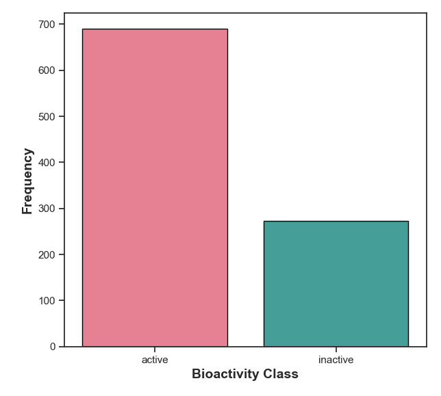


Figure 7: Frequency distribution of active and inactive compounds. The active compounds indicate potential candidates for further development.
Figure 7: Frequency distribution of active and inactive compounds. The active compounds indicate potential candidates for further development.
Feature Engineering
Feature Engineering
In the feature engineering phase I wrote the padel.py script to calculate the PaDEL descriptors, which are critical in capturing the chemical properties of compounds. First the dataframe is cleaned and formatted into a .smi file to ensure compatibility with the PaDEL-Descriptor tool. The PaDEL descriptor is then run to generate a comprehensive set of molecular descriptors for each compound. This provides the foundation for building a predictive model that can learn patterns related to compound activity.
In the feature engineering phase I wrote the padel.py script to calculate the PaDEL descriptors, which are critical in capturing the chemical properties of compounds. First the dataframe is cleaned and formatted into a .smi file to ensure compatibility with the PaDEL-Descriptor tool. The PaDEL descriptor is then run to generate a comprehensive set of molecular descriptors for each compound. This provides the foundation for building a predictive model that can learn patterns related to compound activity.
Model Development
Model Development
In the model building phase I wrote a script, regmodel.py, that trains and evaluates regression models for predicting bioactivity based on the previously generated descriptors. This script streamlined the process of model training, testing, and selection, focusing of accuracy and model comparison to determine the best approach.
First I split the data into training and testing sets using a 80/20 split. Then I moved on to train a Random Forest model, as it is robust and able to capture complex relationships. The calculated R-squared value landed on 0.607 - a moderate fit, i.e. the Random Forest model captures about 61% of the relationships within the data. Next, LazyPredict was used to compare different regression algorithms, both linear models and more complex ones. To visualize the model performance, the script generates several plots, including a scatter plot of predicted vs. experimental pIC50 values for the Ranodm Forest model. Additionally, bar plots of R-squared scores and RMSE values were created.
Results Analysis
Results Analysis
In the model building phase I wrote a script, regmodel.py, that trains and evaluates regression models for predicting bioactivity based on the previously generated descriptors. This script streamlined the process of model training, testing, and selection, focusing of accuracy and model comparison to determine the best approach.
First I split the data into training and testing sets using a 80/20 split. Then I moved on to train a Random Forest model, as it is robust and able to capture complex relationships. The calculated R-squared value landed on 0.607 - a moderate fit, i.e. the Random Forest model captures about 61% of the relationships within the data. Next, LazyPredict was used to compare different regression algorithms, both linear models and more complex ones. To visualize the model performance, the script generates several plots, including a scatter plot of predicted vs. experimental pIC50 values for the Ranodm Forest model. Additionally, bar plots of R-squared scores and RMSE values were created.
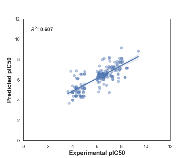


Figure 8: RandomForestRegressor model. The scatter plot shows the predicted versus experimental pIC50 values with a R-squared value of 0.607. An R-squared value of 0.607 means that approximately 60.7% of the variance in the experimental pIC50 values is explained by the RandomForestRegressor model's predictions. This suggests that the model has some predictive power but is not highly accurate, as a substantial portion of the variance remains unexplained.
Figure 8: RandomForestRegressor model. The scatter plot shows the predicted versus experimental pIC50 values with a R-squared value of 0.607. An R-squared value of 0.607 means that approximately 60.7% of the variance in the experimental pIC50 values is explained by the RandomForestRegressor model's predictions. This suggests that the model has some predictive power but is not highly accurate, as a substantial portion of the variance remains unexplained.
R-squared Model Comparison
In this R-squared comparison chart, the models are ranked based on their R-squared values from training data. RandomForestRegressor is near the top but is outperformed by models like DecisionTreeRegressor, ExtraTreeRegressor, ExtraTreesRegressor, GaussianProcessRegressor, and XGBRegressor. These models show slightly higher values compared to RandomForestRegressor.
The DecisionTreeRegressor, ExtraTreeRegressor, and ExtraTreesRegressor models show the highest R-squared values in this chart, suggesting they may provide better predictions on this training dataset. However, the model choice should also consider potential overfitting, as a high R-squared on training data does not always translate to strong performance on test data. It may be worthwhile to further test and validate the top-performing models on separate test data to ensure their generalizability.
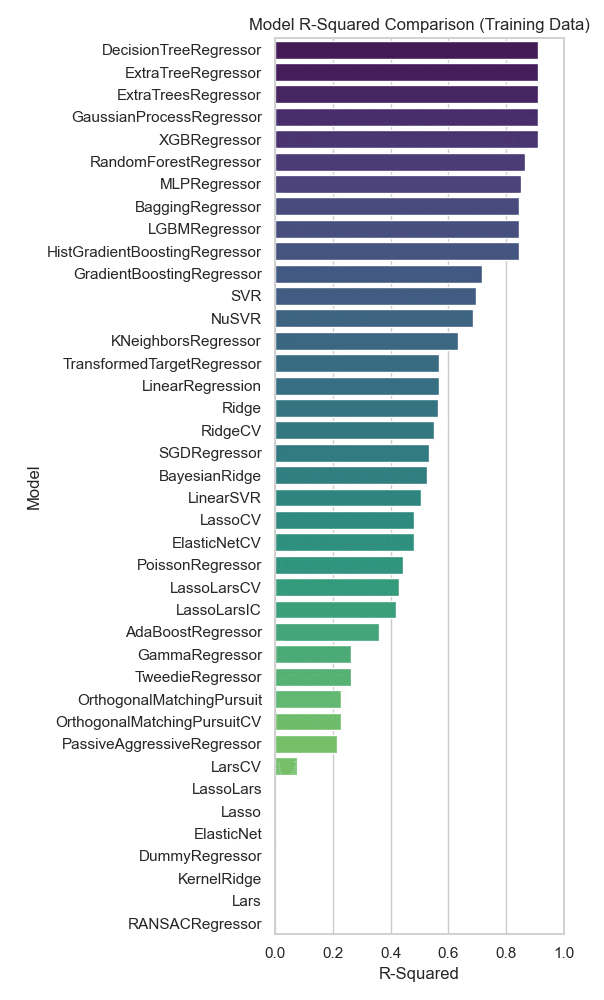


Figure 9: R-squared value comparison between regression models on training data. The models explaining the most variance are DecisionTreeRegressor, ExtraTreeRegressor, ExtraTreesRegressor, GaussianProcessRegressor and XGBRegressor.
Figure 9: R-squared value comparison between regression models on training data. The models explaining the most variance are DecisionTreeRegressor, ExtraTreeRegressor, ExtraTreesRegressor, GaussianProcessRegressor and XGBRegressor.
RMSE plots
By comparing the RMSE values on training and test data for the regression models, we can evaluate both their performance and generalizability. The models with the lowest RMSE on training data are DecisionTreeRegressor, ExtraTreeRegressor, ExtraTreesRegressor, and GaussianProcessRegressor, as seen in Figure 10. On the test data, the RandomForestRegressor, HistGradientBoostingRegressor, LGBMRegressor, and XGBRegressor show the lowest RMSE values, seen in Figure 11. These models perform better on unseen data, indicating that they generalize well and are less prone to overfitting. Models like DecisionTreeRegressor and ExtraTreeRegressor have low RMSE on training data but much higher RMSE on test data, suggesting they are overfitting. They capture noise in the training data but fail to generalize to new data.
The RandomForestRegressor and Gradient Boosting models (including HistGradientBoostingRegressor and XGBRegressor) show balanced RMSE on both training and test datasets. This indicates they are effective at capturing patterns in the data without overfitting, making them more reliable choices. While models like DecisionTreeRegressor excel in training data, the RandomForestRegressor, HistGradientBoostingRegressor, and XGBRegressor appear to be the best overall choices for prediction based on RMSE data, as they perform consistently across both datasets and demonstrate good generalizability.
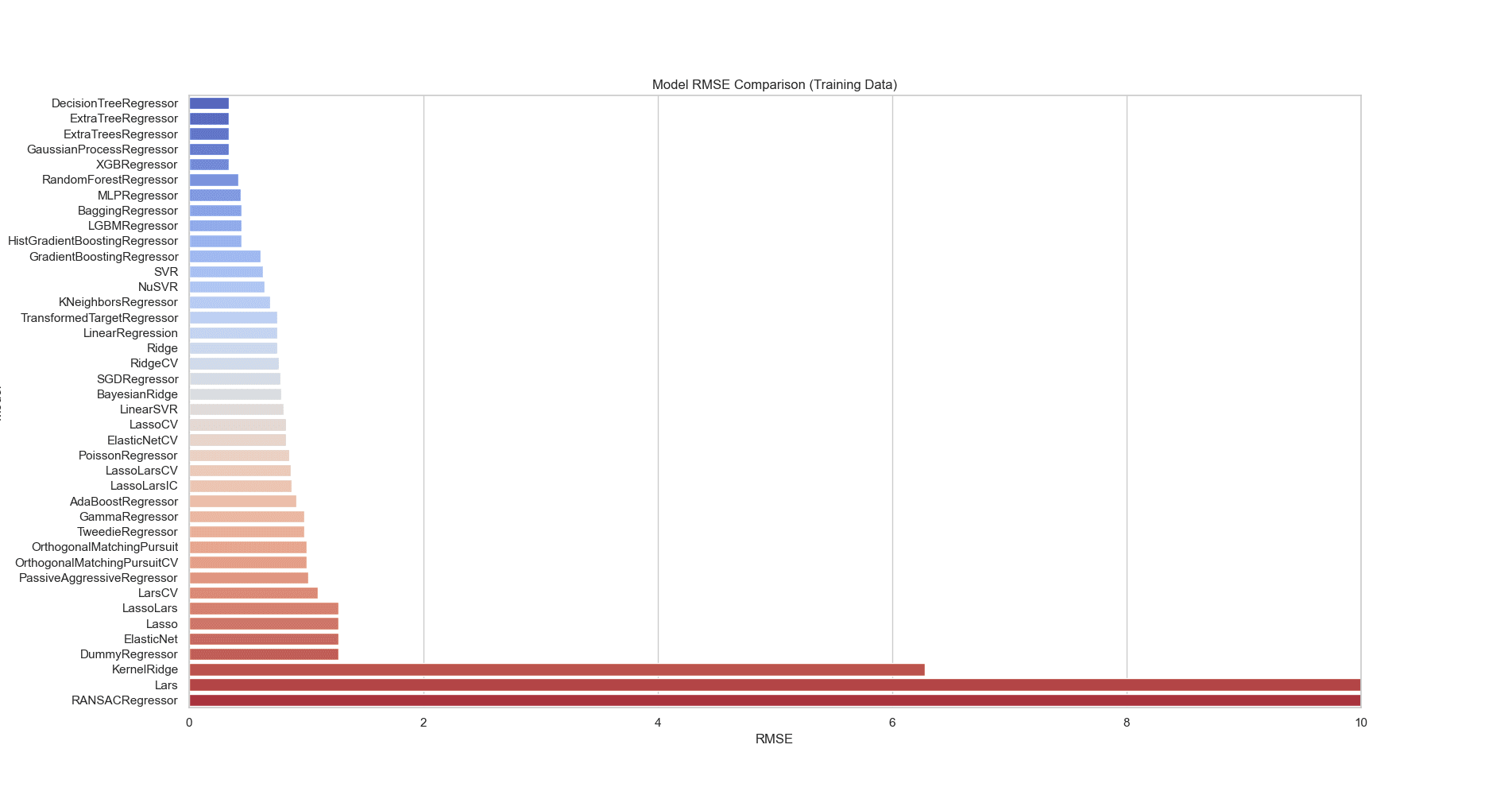


Figure 10: RMSE bar plot comparing different regression models on training data. By comparing the RMSE values on training data for the regression models we can evaluate both their performance and generalizability. The models with the lowest RMSE on training data are DecisionTreeRegressor, ExtraTreeRegressor, ExtraTreesRegressor, and GaussianProcessRegressor.
Figure 10: RMSE bar plot comparing different regression models on training data. By comparing the RMSE values on training data for the regression models we can evaluate both their performance and generalizability. The models with the lowest RMSE on training data are DecisionTreeRegressor, ExtraTreeRegressor, ExtraTreesRegressor, and GaussianProcessRegressor.
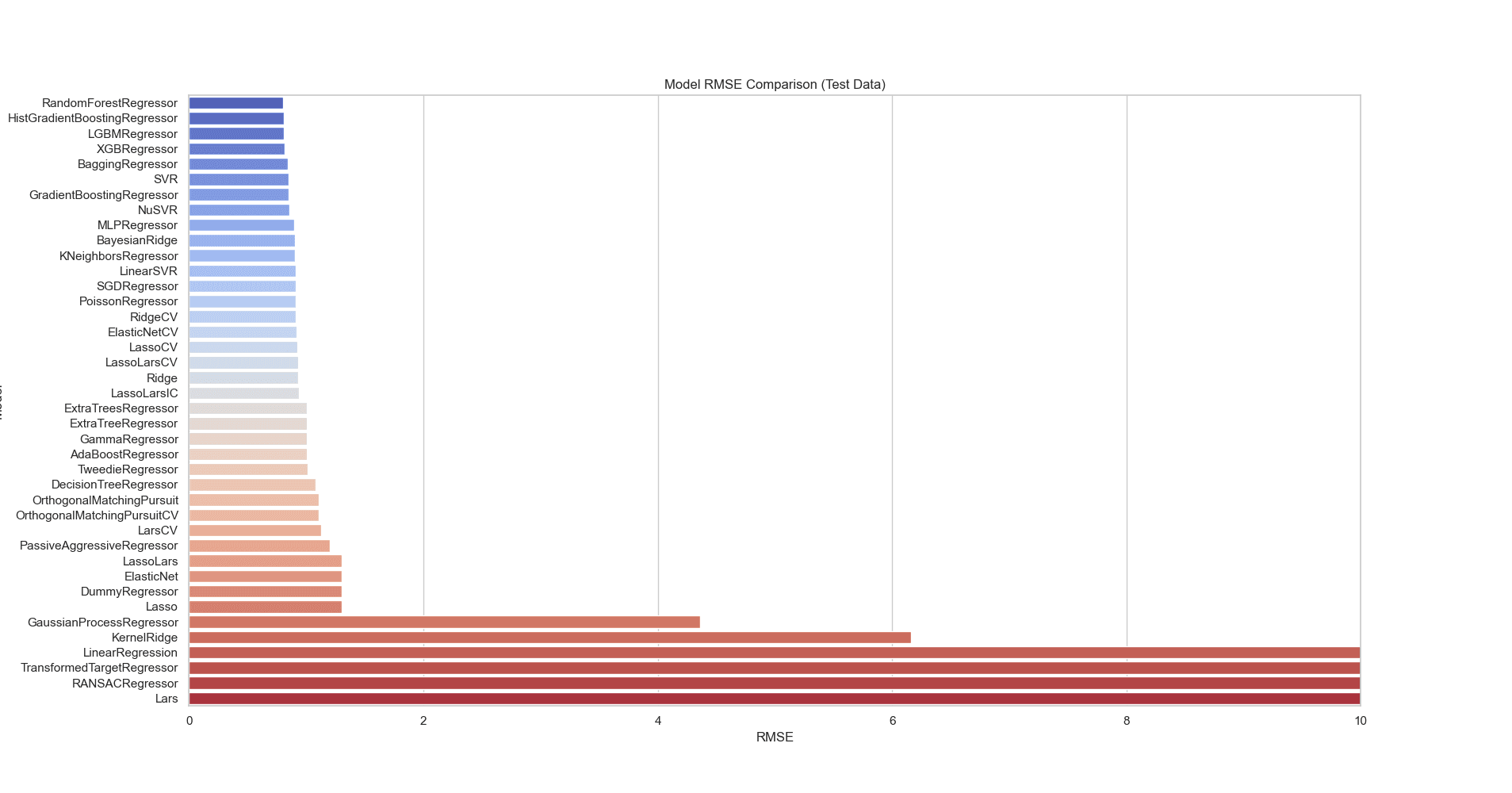


Figure 11: RMSE bar plot comparing different regression models on test data. The RandomForestRegressor, HistGradientBoostingRegressor, LGBMRegressor, and XGBRegressor show the lowest RMSE values. These models perform better on unseen data, generalizing well and less prone to overfitting.
Figure 11: RMSE bar plot comparing different regression models on test data. The RandomForestRegressor, HistGradientBoostingRegressor, LGBMRegressor, and XGBRegressor show the lowest RMSE values. These models perform better on unseen data, generalizing well and less prone to overfitting.
Time Taken
Using the training data, the RandomForestRegressor and ExtraTreesRegressor have relatively short training times compared to models like ElasticNetCV and LassoCV, which take significantly longer, seen in Figure 12. Models like DecisionTreeRegressor and ExtraTreeRegressor are also very efficient, requiring minimal training time.
On test data, RandomForestRegressor and XGBRegressor remain relatively efficient, seen in Figure 13. Models like ElasticNetCV and LassoCV still require considerable time, making them less ideal for scenarios where fast predictions are needed.
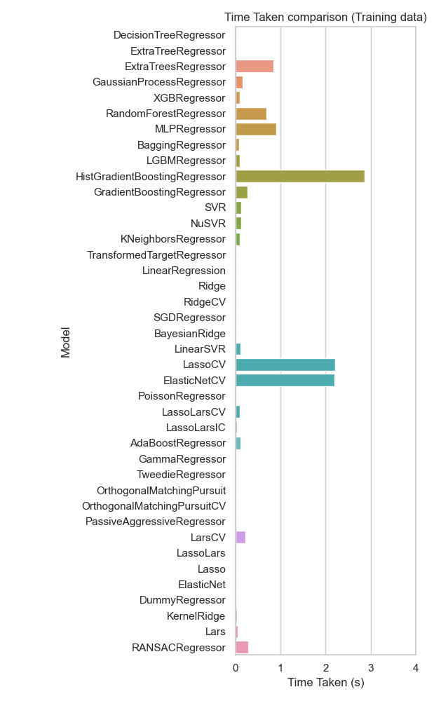


Figure 12: Time taken bar plot comparing different regression models on training data. RandomForestRegressor and ExtraTreesRegressor have relatively short training times compared to models like HistGradientBoostingRegressor, ElasticNetCV and LassoCV.
Figure 12: Time taken bar plot comparing different regression models on training data. RandomForestRegressor and ExtraTreesRegressor have relatively short training times compared to models like HistGradientBoostingRegressor, ElasticNetCV and LassoCV.
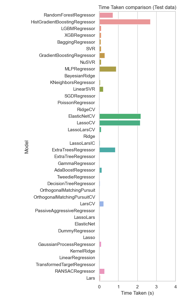


Figure 13: Time taken bar plot comparing different regression models on test data. RandomForestRegressor and XGBRegressor remain relatively efficient. Models like ElasticNetCV and LassoCV still require considerable time, making them less ideal for scenarios where fast predictions are needed.
Figure 13: Time taken bar plot comparing different regression models on test data. RandomForestRegressor and XGBRegressor remain relatively efficient. Models like ElasticNetCV and LassoCV still require considerable time, making them less ideal for scenarios where fast predictions are needed.
Conclusion
Conclusion
RandomForestRegressor strikes a good balance between prediction accuracy, generalizability, and computational efficiency. It has a low RMSE on test data, demonstrating good predictive power and quick training and testing times, making it a strong choice.
HistGradientBoostingRegressor and XGBRegressor also perform well in terms of RMSE but may take slightly longer in training or testing, particularly for HistGradientBoostingRegressor. If the computational cost is not a primary concern, these models are also excellent choices.
Given the overall balance of performance and efficiency, RandomForestRegressor would be a suitable model. It provides accurate predictions, generalizes well to test data, and is efficient in terms of time taken for both training and testing. If additional accuracy is desired and computation time is not a limiting factor, HistGradientBoostingRegressor or XGBRegressor could also be considered, though they may require a bit more computational time. In summary, RandomForestRegressor is recommended as it offers the best combination of predictive performance and computational efficiency.
Beyond these specific results, this project highlights the value of integrating cheminformatics tools and predictive modeling to streamline compound screening. By leveraging ChEMBL data, performing detailed exploratory data analysis, and using advanced feature descriptors (PaDEL), I was able to develop and evaluate models that can significantly aid in identifying potential inhibitors. This approach not only accelerates the drug discovery timeline but also reduces the need for costly and time-consuming experimental assays in early research stages.
If any questions arise, feel free to contact me personally.


